Node Voltage Analysis in Electric Circuits

In nodal analysis, Kirchhoff’s Current Law is used to write the equilibrium equations.

A node is defined as a junction of two or more branches.

If we define one node of the network as a reference node (a point of zero potential or ground), the remaining nodes of the network will have a fixed potential relative to this reference.

Equations relating to all nodes except the reference node can be written by applying KCL.

---

Reference Node

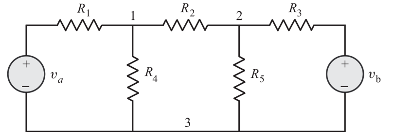
Referring to the circuit shown in Figure, we can arbitrarily choose any node as the reference node. However, it is convenient to choose the node with the most connected branches.

Hence, node 3 is chosen as the reference node here.

It is seen from the network that there are three nodes.

Hence, the number of equations based on KCL will be:

$$\text{Number of node equations} = \text{Total number of nodes} - 1$$

Therefore, in the present case, we will have only two node equations.

---

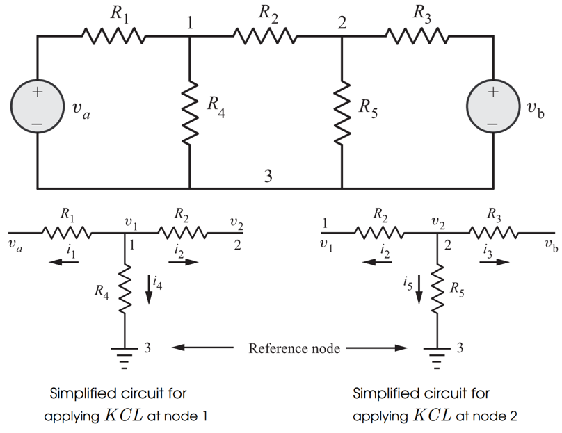
Applying Kirchhoff’s Current Law

For applying KCL at node 1 and node 2, we assume that all currents leave these nodes.

Applying KCL at node 1:

$$\frac{v_1 - v_a}{R_1} + \frac{v_1 - v_2}{R_2} + \frac{v_1}{R_4} = 0$$

Applying KCL at node 2:

$$\frac{v_2 - v_1}{R_2} + \frac{v_2 - v_b}{R_3} + \frac{v_2}{R_5} = 0$$

Rearranging the equations,

$$\left( \frac{1}{R_1} + \frac{1}{R_2} + \frac{1}{R_4} \right)v_1 - \frac{1}{R_2}v_2 = \frac{v_a}{R_1}$$ $$- \frac{1}{R_2}v_1 + \left( \frac{1}{R_2} + \frac{1}{R_3} + \frac{1}{R_5} \right)v_2 = \frac{v_b}{R_3}$$

---

Matrix Form of Node Equations

Putting the above equations in matrix form, we get:

$$\begin{bmatrix} \frac{1}{R_1}+\frac{1}{R_2}+\frac{1}{R_4} & -\frac{1}{R_2} \\ -\frac{1}{R_2} & \frac{1}{R_2}+\frac{1}{R_3}+\frac{1}{R_5} \end{bmatrix} \begin{bmatrix} v_1 \\ v_2 \end{bmatrix} = \begin{bmatrix} \frac{v_a}{R_1} \\ \frac{v_b}{R_3} \end{bmatrix}$$

---

Solving Node Equations Using Cramer’s Rule

Step 1: Find the Determinant

The determinant of the coefficient matrix is:

$$\Delta = \begin{vmatrix} \frac{1}{R_1}+\frac{1}{R_2}+\frac{1}{R_4} & -\frac{1}{R_2} \\ -\frac{1}{R_2} & \frac{1}{R_2}+\frac{1}{R_3}+\frac{1}{R_5} \end{vmatrix}$$

---

Step 2: Find Determinant for (v_1)

Replace the first column with constants:

$$\Delta_1 = \begin{vmatrix} \frac{v_a}{R_1} & -\frac{1}{R_2} \\ \frac{v_b}{R_3} & \frac{1}{R_2}+\frac{1}{R_3}+\frac{1}{R_5} \end{vmatrix}$$

Therefore,

$$v_1 = \frac{\Delta_1}{\Delta}$$

---

Step 3: Find Determinant for (v_2)

Replace the second column with constants:

$$\Delta_2 = \begin{vmatrix} \frac{1}{R_1}+\frac{1}{R_2}+\frac{1}{R_4} & \frac{v_a}{R_1} \\ -\frac{1}{R_2} & \frac{v_b}{R_3} \end{vmatrix}$$

Therefore,

$$v_2 = \frac{\Delta_2}{\Delta}$$

Once (v_1) and (v_2) are obtained, all branch currents can be found using Ohm’s law.

Thus, the complete solution of the network is obtained.

---

Summary

• Node voltage analysis is based on Kirchhoff’s Current Law.
• One node is selected as the reference or ground node.
• The number of node equations is equal to total nodes minus one.
• Node voltages are solved using simultaneous equations.
• Cramer’s rule can be used to solve node equations systematically.